FIG PUBLICATION NO. 49Cost Effective GNSS Positioning TechniquesFIG Commission 5 PublicationDr. Neil D. Weston, United States
|
 |
|
|
 |
This publication as a .pdf-file (46 pages - 1.22 MB) |
2. Global Navigation Satellite Systems
2.1 Introduction
2.2 GPS
2.2.1 Introduction
2.2.2 GPS Signal Structure
2.2.3 GPS System Time
2.3 GLONASS
2.3.1 Introduction
2.3.2 Signal Structure
2.3.3 GLONASS in the Future
2.4 GALILEO
2.4.1 Introduction
2.4.2 Galileo Signals
2.4.3 Galileo Services
2.5 COMPASS
3. GNSS Positioning Techniques for Surveying
3.1 Introduction
3.2 Relative Positioning
3.3 Precise Point Positioning
3.4 Positioning Software Packages and Data Types
4. Cost-effective GNSS
4.1 Introduction
4.2 Cost-Effective Rovers / Low-Cost GNSS Receivers
4.3 Continuously Operating Reference Station (CORS) Networks
4.3.1 Introduction
4.3.2 CORS Station Configuration
4.3.3 Products from a CORS Network
4.4 Web-based Positioning Tools
4.4.1 Online Positioning User Service
– OPUS
4.4.2 Scripps Coordinate Update Tool –
SCOUT
4.4.3 AUSLIG’s Online GPS Processing
Service – AUSPOS
4.4.4 Canadian Spatial Reference System
Online Global GPS Processing Service – CSRS-PPP
Appendix A - The International GNSS
Service
Appendix B - Additional Information and Resources
Appendix C - Global and Regional Reference Station
Networks
Most surveyors today are aware that data acquisition, management, analysis, presentation and controlling systems are becoming more elaborate and automated. The International Federation of Surveyors (FIG) Commission 5 – Positioning and Measurement, has been and remains an essential part of the surveying community’s growth and development. During the past decade, Global Navigation Satellite Systems (GNSS) have and continue to play an increasingly important role in positioning and navigation.
The FIG enhances this development by facilitating GNSS sessions at their conferences, encouraging GNSS research and education, and cooperating with sister organisations such as the International Association of Geodesy (IAG) in the respective domain. Additionally, the FIG is also trying to integrate GNSS surveying as a base and starting point for land administration as well as cadastral registration, especially in developing countries regarding property evidence. This is one of the major reasons why FIG is looking at cost-effective technologies and techniques for enabling surveyors in developing countries to use the best equipment at a reasonable price. This Technical Report focuses on the cost-effective use of GNSS. It originates with the help of Special Study Group “Cost-Effective GNSS” within the Working Group 5.4 “GNSS”.
As Chair of FIG Commission 5 – Positioning and Measurement, I thank Dr. Neil Weston, National Geodetic Survey, USA and Dr. Volker Schwieger, University of Stuttgart, Germany for their efforts in compiling this report.
| Prof. Dr.-Ing. Rudolf Staiger Chair FIG Commission 5 January 2010 |
Global Navigation Satellite Systems (GNSS) were initially developed in the early seventies to improve global positioning and navigation from space. The Global Positioning System (GPS) was the first system to launch an operational prototype satellite in February of 1978. Shortly after, the number of GPS satellites in orbit increased to four but this was the absolute minimum to obtain a “fix”. More satellites would be needed if continuous global coverage was expected. GNSS constellations are constantly being expanded and upgraded but many of the initial designs and integrated systems on the original satellite are still found on newer satellites in the current GPS constellation.
The first commercial GPS receivers were on the market in 1982. The receivers were large and bulky and could only track four satellites simultaneously. The satellites to track had to be selected manually on the receiver. Moreover, national geodetic agencies, research institutions and universities spent up to 250,000 € for a single receiver. Today, modern receivers are much more sophisticated and can track GPS and GLONASS satellites simultaneously on more than 50 channels. Some of the latest receiver models can also track Galileo signals. Everything from satellite tracking to coordinate determination are computed automatically in real time. At the same time costs of new receivers continue to decrease. A high-end geodetic quality GNSS receiver costs around 20,000 €. If a user is restricted to single-frequency, geodetic quality receivers, one would still have to spend 5,000 € to 12,000 €. In general this does not pose a problem in developed countries, but it may be a drawback in developing countries or for tasks where the surveyor needs a lot of receivers for specialized tasks such as monitoring.
In this FIG report the authors will present several topics on the
cost-effective use of GNSS. There are two possibilities to economize resources.
The first pertains to a reference site or a network of reference stations and
the second primarily concentrates on the rover or users side. For the first, we
initially focus on Continuously Operating References Station (CORS) networks
that provide the reference site(s) data and metadata to the users. For the
second, the report proposes to use low-cost (below 150 €) GNSS receivers instead
of high-end geodetic quality receivers. After giving an overview on GNSS and
geodetic positioning, both approaches and their opportunities are presented.
Finally, several cases on estimating the working costs will be developed and
analyzed.
In the modern age of positioning and navigation, satellites from any of the Global Navigation Satellite Systems (GNSS) can be used to accurately position stationary or moving objects. This general approach is often termed satellite positioning. The basic idea is to determine the position of an antenna (Ri(t)) connected to a GNSS receiver where the antenna could be over a survey marker, on a plane or ship, or even be a part of a GNSS reference network. Since the positions of all the satellites in a constellation can be calculated at any time t and the range between any visible satellite and the antenna is measured by a GNSS receiver (ρj i(t)), the only remaining unknown is the position vector from the origin of a common coordinate system to the antenna which is being positioned. Fig. 1 shows the basic concept of satellite positioning using a single satellite j and an Earth Centered Earth Fixed (ECEF) reference frame.
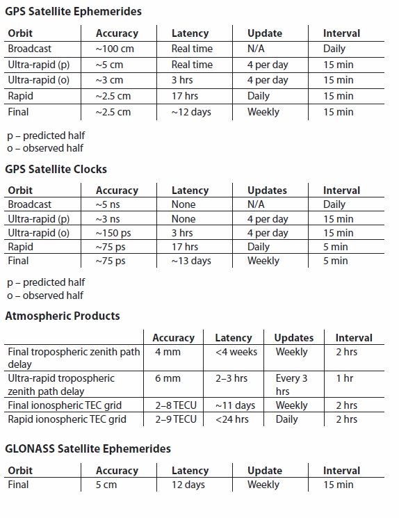
In practice however, accurate positioning of objects with GNSS satellites is much more complex. If we look at a constellation of satellites first, a user needs to know the exact position of each of the space vehicles (Rj(t)) during a period of time or in the near future. Satellite positions as a function of time, otherwise known as ephemerides, were initially determined by groups working in spacecraft dynamics, aeronautics and celestial mechanics. Today there are quite a few research and academic institutions which are actively involved in computing satellite ephemerides. The International GNSS Service (IGS), for example, uses a global network of reference stations to track the position and estimate the orbit of each satellite using a weighted least squares process (Beutler et al. 1999, 2005, 2009, Dow et al. 2009, Appendix B.1–2). Over the last decade, the orbit determination process at the IGS Analysis Centers has improved significantly and accuracies better than a few centimeters for the IGS Rapid and Final orbit products are now routinely achieved. Appendix A lists the orbit products and their accuracies which are currently available through the IGS.
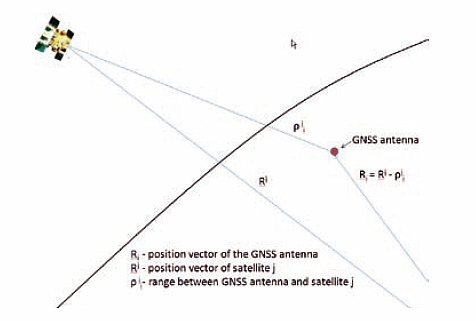
Fig. 1: Satellite positioning using an ECEF reference frame.
Another major area for discussion has to do with how the range (ρj i(t)) between satellite j and receiver i is measured. Different positioning techniques have evolved based on various operating conditions, but all use the following basic equation to estimate the position vector Ri(t) for an antenna.
|| Rj(t) – Ri(t) || = ρj i(t) i,j = 1,2,3,... (2.1)
For stationary objects, the most common positioning techniques are precise point positioning (PPP) and relative or differential positioning. For these cases, a user can compute a position every epoch and under ideal conditions, should get redundant results. As a second method, a user could also compute a single set of coordinates based on many epochs, either through averaging or with a least squares approach (Strang and Borre 1997, Leick 2004).
If an antenna is on a moving platform, then a position has to be computed at every epoch and is often referred to as kinematic positioning. Two frequently used techniques under this category are point positioning and real-time kinematic positioning, in either a point positioning mode or relative to one or more stationary receivers. These approaches are often augmented by additional ground or space-based systems such as the wide area augmentation system (WAAS) used primarily by the aviation industry and the differential GPS (DGPS) system initially implemented by the United States Coast Guard.
Many augmentation systems such as the WAAS system use geostationary satellites to broadcast differential correctors to receivers for improving the positioning capabilities as well as enhancing the integrity of the overall system. The Coast Guard’s DGPS system was initially designed to support the maritime communities along the coasts and inland waterways of the United States, but because of its performance and popularity, the system is now being expanded across the nation and is being referred to as the Nationwide Differential Global Positioning System (NDGPS). Similar augmentation systems have also been developed and are currently operational in Europe and Japan. The European Geostationary Navigation Overlay Service (EGNOS) uses three geostationary satellites and numerous ground stations to enhance critical navigation applications used by civilian and military aircraft and ships in Europe. The MTSAT augmentation system being developed by Japan will support the country’s meteorological agency as well as the aviation sectors and will provide coverage over East Asia and the Western Pacific.
The Navigation Satellite Timing and Ranging (NAVSTAR) Global Positioning System (GPS) was developed by the United States Department of Defense (DoD) to provide worldwide positioning and timing capabilities for the military. The system was initially designed to provide two types of services. The first is the precise positioning service (PPS) and is for military use while the second is the standard positioning service (SPS) and is intended for use by everyone (SPS, 2001)
Different components of the GPS system fall into three main groups. The first is known as the SPACE segment and consists of 24 operational satellites built by Rockwell International, Lockheed Martin and Boeing. Four atomic clocks on each satellite continuously compute and transmit the exact time (GPS time) and position of the satellite in a digital signal. The satellites are also placed, in equal numbers, in six orbital planes, each inclined at 55° from the Earth’s equator. Each satellite moves in a near circular orbit (semi-major axis 26,660 km) and completes two orbital revolutions in one sidereal day. The inclination of the orbits and the high altitude (~20,000 km) of the GPS satellites permit more to be seen simultaneously from virtually anywhere on Earth. Satellite visibility is also optimized by monitoring and routinely adjusting the positions of all satellites in each orbital plane.
The second major component of the GPS system is the CONTROL segment. This currently consists of eleven monitoring stations where each station monitors and accumulates the range to each visible satellite before passing the information on to the Master Control Station (MCS) at Schriever AFB in Colorado. The MCS is responsible for computing the orbit of each satellite and to update the navigation or broadcast message with parameters that describe each satellite’s orbit. The broadcast message is then sent to each satellite via an up-link from one of three ground antennas located in Ascension Island, Diego Garcia and Kwajalein.
The third component of the GPS system is the USER segment. This primarily consists of GPS antennas and receivers that provide position, navigation and timing information to the users. The number of applications for GPS continues to rise and over the last decade, there has been a dramatic increase in the number and type of receivers which have been developed and sold for civilian and military uses.
One of the principle design features of all GPS satellites is to use onboard atomic clocks to generate signal transmissions from the fundamental frequency of 10.23 MHz. The two initial signals on all GPS satellites are known as the L1 and L2 carriers and are multiples of the fundamental frequency. The L1 carrier is 154 times the fundamental frequency, f1 = 1575.42 MHz while the L2 carrier is 120 times the fundamental frequency, f2 = 1227.60 MHz. The encrypted Precision or P(Y) codes on the L1 and L2 carriers have the same fundamental frequency of 10.23 MHz, while the Coarse/Acquisition or C/A code has a chipping rate of one-tenth the fundamental frequency, i.e., 1.023 MHz.
As part of the GPS modernisation effort, a second civil frequency was added on L2 for Block IIR-M and later satellites launched after 1998. The new navigation signal is referred to as L2C and aims to improve accuracy of navigation with enhanced signal tracking capabilities. In March 2009, a Block IIR-20(M) satellite was launched with the new L5 safety of life civil signal (1176.45 MHz) and is the first in a series designed with higher transmitting power, wider bandwidth and enhanced performance. The modernisation of the GPS constellation aims to provide more transmitting signals to both the civilian and military communities and is scheduled to continue through 2013.
GPS system time is the time given by the composite clock which
includes monitoring stations and the satellite frequency standard. A master
clock for GPS time is constantly checked against a clock at the United States
Naval Observatory (USNO) and steered to UTC so the difference is no greater than
one microsecond. The navigation message which contains parameters that describe
the satellite orbits also has two parameters that specify the time offset and
the rate of drift between GPS time and UTC (USNO). UTC (USNO) is also
synchronized to be in agreement with the international benchmark
for UTC.
The Global Navigation Satellite System (GLONASS – GLObal’naya Navigatsionnaya Sputnikovaya Sistema) is managed by the Russian Space Forces for the Russian Federation Government. All operational components of the GLONASS system are operated by the Coordination Scientific Information Center (KNITs) which is a part of the Ministry of Defense of the Russian Federation. Initial GLONASS development began in 1976 in the former Soviet Union and was designed to be an alternative to the GPS system offered by the United States. There have been several generations of satellites in the GLONASS constellation. The two most recent, which are known as GLONASS-M and GLONASSK, have an estimated operational life span of 7 and 12 years respectively. All satellites have atomic clocks and provide real time position and velocity determination once a receiver has locked on and remains in signal tracking mode. During the early operational stages, the horizontal positional accuracy varied between 50–70 meters while the vertical accuracy was closer to 70 meters.
The space segment of GLONASS consists of 24 satellite slots in three orbital planes separated by 120° and inclined at 64.8° with respect to the equator. The eight satellite slots in each plane, numbered 1–8 for plane one, 9–16 for plane two etc., have a separation of 45°, a near circular orbit with a period of 11 hours and 15 minutes, and have an altitude of 19,100 km above the Earth. The spatial arrangement of the satellites in the three planes is such that only one crosses the equator at a time and therefore a minimum of five can be seen at any time, from any location on Earth. Any specific GLONASS satellite will therefore pass over the same spot on Earth every eight sidereal days while each GPS satellite passes over the same spot once every sidereal day.
The GLONASS control segment has two primary divisions. The first is the Ground Control Center located in Moscow and the second are the telemetry and tracking stations located at St. Petersburg, Eniseisk, Ternopol and Komsomolsk-na-Amure. The GLONASS operating authorities also have active expansion plans which include additional monitoring and tracking stations in Australia, Cuba and South America to enhance the accuracy, reliability and integrity of the system.
As of January 2010, the GLONASS system consists of 19 operational satellites with two additional satellites listed as „in maintenance“. The Russian territory has complete coverage with 19 satellites but for 100% global coverage with five or more satellites in view, 24 satellites need to be operational.
There are two types of signals which are transmitted from the GLONASS satellites. The first is the standard precision (SP) signal which is transmitted between 316–500 Watts in a 38° cone using right-hand circular polarization. Each satellite transmits the SP signal on the same code but uses a different frequency. The L1 band is used with a technique known as frequency division multiple access (FDMA) to assign different frequencies centered around 1602.0 MHz to 15 channels. The frequencies for the 15 channels are calculated by using the following formula 1602.0 MHz + 0.5625 MHz x n where n is an integer value from –7 to 7. The frequency for channel 0 would therefore be 1602.0 MHz while the frequency for channel –7 would be 1595.56 MHz. The horizontal accuracy, using the SP signal from four older GLONASS (first generation) satellites, was typically between 5–10 meters while the vertical accuracy was about 15 meters.
The second signal known as the high precision (HP) signal shares the same carrier wave as the SP signal but uses a bandwidth which is 10 times larger. The HP signal is primarily used by the Russian military and other sectors with authorized access. The FDMA technique is also used to assign 15 L2 frequencies of the HP signal but now they are centered near 1246 MHz. In this case, the same integer values used for n to calculate frequencies for L1 are used for L2 but with the following formula 1246 MHz + 0.4375 MHz x n. Even though the HP signal was broadcasted in a clear, un-modulated format in the past, caution in using the signal is still suggested because a recently adopted approach to broadcast 400bps at random intervals has been implemented on a permanent basis.
A fairly significant change to parts of the GLONASS signal structure are scheduled to take place when GLONASS-K (third generation) satellites are added to the current constellation. These satellites will use code division multiple access (CDMA) for L1 and L5 signals, a technology which employs a coding scheme where each transmitter is assigned a unique code so numerous users can be multiplexed over the same physical channel. The CDMA approach will also begin to make the GLONASS constellation more compatible with GPS and the future Galileo system.
Galileo is formally known as the European Civil Satellite Navigation Program and its start can be traced back to March, 2002 when the European Council voted to declare the program as an official undertaking. The Galileo Program has received most of its initial funding from numerous public and private European institutions and is currently being developed as an inter-operable counterpart to the GPS and GLONASS systems offered by the United States and Russia.
The Galileo system is being designed with several major operational segments. The first or global segment will contain 30 Medium Earth Orbit (MEO) satellites, 27 operational and three spare, in three orbital planes inclined at 56˚. In-plane satellites will be positioned at 40˚ intervals, have an altitude of 23,222 km and will be maneuvered via velocity changes so orbit period fluctuations are kept to an absolute minimum. The orbits were also chosen to minimize gravitational resonances and to provide high visibility of the satellites. Each satellite will transmit up to 10 navigation timing and data signals, some of which will contain clock and ephemeris information to enable worldwide positioning, navigation, timing and integrity monitoring services.
The ground control segment will be made up of five up-link stations located around the world and will be responsible for the telemetry, tracking and command (TTC) tasks for communicating with the satellites on a regular basis. Two additional control centers located in Oberpfaffenhofen, Germany and Rome, Italy will be responsible for analyzing and initiating spacecraft control functions via the five TTC stations. Orbit maintenance and systems monitoring activities will also be performed at the two European control centers. A larger global network of up to 30 tracking stations will be used to continuously monitor all satellite navigation signals in a redundant fashion.
Another significant component of the Galileo infrastructure is the regional segment which will consist of numerous agencies within and outside Europe that will offer integrity services independent of the Galileo system. The integrity services, known as External Region Integrity Systems (ERIS), will also be a part of a checking system used to legally monitor products, services and guarantees offered by Galileo.
Each satellite in the Galileo constellation will use CDMA technology to transmit up to 10 right hand circular polarized signals in the frequency ranges 1164–1592 MHz. A specific code or key is added to each signal so receivers can identify which satellite the signals are coming from and how long the transmissions took. The more complex the code, the more time a receiver spends in identifying which channel to assign for the signal. The satellite identification codes also come in two formats. A long format code is more difficult to acquire but improves tracking capabilities when signals are very weak while short codes allow for very fast acquisitions.
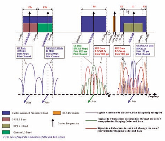
Fig. 2: Galileo Signal Structure. (Courtesy Institute of Geodesy and
Navigation, University FAF Munich)
The range of the E5a band is 1164–1189 MHz and has 1176.45 MHz as its central frequency. The same range is also used for the GPS L5 signal. The E5b band is 1189–1214 MHz and uses 1207.14 MHz as the main frequency. This band is equivalent to the GLONASS L3 band. The data on signals from the E5a and E5b bands are partly encrypted and is available to all users.
The multi-lobed E6 band from 1260–1300 MHz is unique to Galileo. It uses 1278.75 MHz as the central frequency to transmit signals which have controlled access to the encrypted range and data information. Signals associated with the side lobes of the E6 band are also encrypted and have restricted access to the range and data information.
The final block of frequencies contain the E2, L1 and E1 signals. This band ranges from 1559–1592 MHz, has a central frequency of 1575.42 MHz and is used by both GPS and Galileo for the L1 signal. Figure 2 summarizes the frequency spectrum, signal structure and data rates used by GPS and Galileo.
One of the main reasons Galileo will offer up to 10 signals is to try to meet the demands and requests brought forward by many current and future GNSS users. Improving signal acquisition, tracking signals indoors, providing codes with different signal characteristics and trying to improve the techniques used to estimate the ionospheric delay are specific cases that would benefit from having more signals. The signal structures and frequency allocations were chosen by design so signals could be used in pairs, such as in determining the ionospheric delay, where measurements using two different signals from the same satellite can be determined and cancelled out. This effect is even more pronounced as the separation between the frequencies of the two signals increases.
With respect to common services such as positioning and navigation, GPS and Galileo will have the same L1 and L5 signals and therefore any increase in the number of satellites in space will strengthen the geometry used to obtain a position.
In addition to the common services, there will be four or five Galileo satellite-only services offered worldwide. The Open Service (OS) provides position and timing capabilities, free of charge, to the worldwide community. The performance of this service is on par with similar services offered by other satellite constellations. The Public Regulated Service (PRS) uses two signals and is offered to specific users who use high performance positioning and timing applications that demand long continuity of service. The Commercial Service (CS) offers similar features to select users but the signals used in this case offer higher throughput rates and will be tailored for high accuracy applications. The Safety of Life Service is designed to improve the Open Service by providing integrity messages when performance falls below a specified threshold. The last signal to be discussed in this section is the Search and Rescue Service. Each Galileo satellite will be able to detect a distress signal and pass on its location to a monitoring center in near-real time thereby enabling rescue services more quickly. An acknowledgement or feedback, in some cases, could be sent to two-way emergency beacons.
The United States, Russia and the European Community are not the only countries to enter the global navigation and positioning race. China is also developing an independent system to operate on a worldwide basis. Their initial system is known as Beidou-1 and consists of four geostationary satellites positioned primarily over Asia. Two satellites were launched in late 2000, a third in 2003 and the fourth in 2007. The experimental constellation provides limited coverage that ranges from 70° E to 140° E and from 5° N to 55° N. However two of the satellites are not usable and the status of a third is unclear.
China’s new system known as Compass or Beidou-2 will have a constellation of 35 satellites, will provide worldwide positioning and navigation capabilities and will offer two levels of service. Five satellites will be geostationary so the system is backward compatible with Beidou-1 while the remaining satellites will reside in medium Earth orbits. The transmitting signals will be based on code division multiple access (CDMA) technology and will use frequencies from the E1, E2, E5B and E6 bands.
As of early 2009 two Compass satellites have been launched. Compass-M1 was placed in orbit for testing of signals from the E2, E5B and E6 bands and to validate a number of service systems. A third Compass satellite was later launched on January 17th of 2010. Implementation of a regional version of the Compass GNSS system with 12 satellites is currently underway and is scheduled to be complete by 2012. Funding to complete and operate the 35 satellite constellation by 2020 has been assured.
Positioning of benchmarks and other stationary objects is routinely referred to as static positioning while the positioning of moving platforms such as a plane or a ship is referred to as kinematic positioning. Since this report mainly addresses surveying, the authors will primarily focus on static applications. Nevertheless kinematic problems may be solved in a similar way. One very important point to note is that surveying applications need accuracies that range between a few centimeters and a few millimeters. This implies that phase observations have to be evaluated and each of the ambiguities have to be solved. In this paper we cannot discuss all aspects of GNSS positioning, however numerous textbooks are available to address advanced topics. In the following sections, information regarding relative positioning and precise point positioning are addressed since background information on these topics are needed to understand the cost-effective techniques in chapter four. Two additional topics will be addressed at this time. The first is that the measurement quantities are referred to as pseudo-ranges since the ranges are affected by the receiver clock error resulting in a pseudo-range. The pseudo-ranges may be determined using code or carrier phase data. The term pseudorange however, does not provide any decision with respect to how the code or phase measurements were used, it is simply a general term. The second point to mention is that a minimum of four pseudo-ranges are needed to determine the position of an antenna, three for the coordinates and one for the receiver clock error. This implies that a minimum of four satellites have to be tracked simultaneously at each receiver-antenna combination to obtain a position at each epoch.
The absolute accuracy of GNSS is about three to four meters if the broadcast navigation message is used for positioning. In this case the positions are determined with respect to the predicted satellite orbits. The satellite broadcast elements are transferred to the user in real time via the broadcast message which are modulated and transmitted on the GNSS signals. This simplest positioning technique is known as absolute GNSS. This technique will never reach the accuracy required for surveying tasks. There are two approaches to obtaining highly accurate surveying results. The first is to use the carrier phase data instead of the code data and the second is the use of differences between measured pseudo-distances. The second technique is known as relative or differential GNSS (DGNSS). If phase data is used we generally refer to this technique as precise DGNSS. Common abbreviations are PDGNSS and PDGPS, but it depends on which constellations are being used for the technique. The main error sources of GNSS have to be identified to understand the advantages of differencing. The principle error sources are associated with satellite orbits, satellite clocks, ionosphere, troposphere, multipath, receiver clock and the antenna phase centre. Figure 3 shows these main sources.
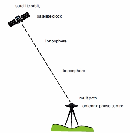
Fig. 3: GNSS main error sources.
The theory behind differential GNSS is the assumption that the errors are more or less the same as long as the pseudo-ranges have similar paths from the GNSS antenna site to the satellite. As an example, pseudo-ranges from two sites separated by less than 50 km to the same satellite will probably have similar atmospheric conditions and therefore similar errors. The paths through the troposphere and the ionosphere are more or less the same with respect to the satellite orbit and geometry. This holds true since the distances to the satellites are more than 20,000 km compared to a 50 km separation or less for two stations on the ground.
The first step in differential GNSS is the generation of single-differences (Figure 4). In this example, a pseudo-range from site one P1 to satellite one S1 is subtracted from the pseudo-range from site two P2 the same satellite S1. Using this technique the error sources associated with the satellite orbit, satellite clock, ionosphere and troposphere are reduced or even eliminated if the same identically oriented antennas are used on both sites. Although most of the errors have been reduced, most of the software packages difference a second time. Here the single-differences are differenced a second time to get a double-difference (Figure 5). The single-difference to satellite one S1 is subtracted from the single-difference to satellite two S2. Using this approach, the influence of troposphere and ionosphere are further reduced and the receiver clock error is eliminated.
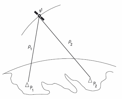
Fig. 4: Single-difference.
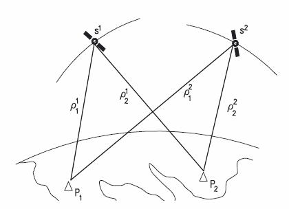
Fig. 5: Double-difference.
If one uses double-differences as measurements in an adjustment procedure, the relative coordinates between the two sites can be determined. To get absolute coordinates in the World Geodetic System 1984, (WGS84) – the GPS coordinate system or the International Terrestrial Reference Frame (ITRF), coordinates of one of the two sites have to be known. In general the respective site is called a reference or base station. The second station, for which the coordinates will be determined, is called the rover. The reference site may be a single reference site or even a large network of GNSS reference sites (see Section 4.3). The second approach is significantly more accurate and reliable. Additionally, it should be mentioned that this technique was originally developed for post-processing but is now frequently used in real time positioning.
In chapter 3.2 the authors emphasized the importance of relative GNSS positioning to meet survey specifications. During the last few years a technique that relies on absolute positioning was developed and continues to gain in importance – precise point positioning (PPP). The elimination of errors by differencing is replaced by precisely modeling many of the error sources. The coordinates of a site are determined with respect to the orbits of the satellites, similar to absolute positioning, but the orbits are known with a high level of accuracy (within a few cms). The same is valid for the satellite clocks (up to sub-nsec). Table 1 gives an overview of the different orbit classes generated by the International GNSS Service (IGS) (see Appendix A). Obviously the highest accuracy may be achieved using the IGS final products where the accuracy of the orbit class improves over time (predicted, rapid, final). This is one reason why highly accurate results are only possible in post-processing modes. Results in real time or near real time are published, but so far the accuracy of the solutions and the reliability of the techniques do not approach the level needed by many surveying applications.
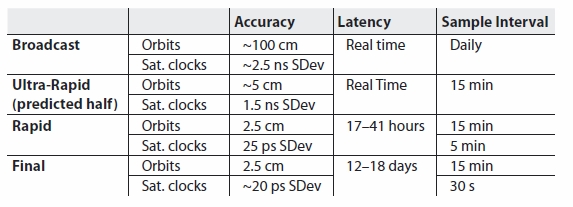
Tab. 1: Orbits and clocks provided by the IGS, broadcast for comparison.
Now returning back to the exact models, three error sources that require special attention are due to the ionospheric and tropospheric influences as well as receiver antenna phase patterns. Additionally, there are error sources that are completely eliminated by using double-differences or absolute GNSS techniques. Some errors are less importance for PDGNSS because they have no effect on the accuracy level. Special attention should also be given to phase centre offsets and variations of the satellite antennas, the phase wind-up at the satellites, the solid earth tides as well as ocean loading effects.
Table 2 gives an overview on several large error sources and their influences on the positioning result. These errors can be modeled and thus the accuracy of PPP using phase measurements is comparable to PDGNSS. The only disadvantage is that the measurement times need to be longer than in PDGNSS because each of the different parameters of the models have to be estimated. Measurement times of 30 minutes are typically required to reach PDGNSS accuracy levels (convergence time). The main reason for this pertains to the tropospheric parameters.
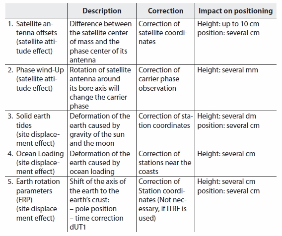
Tab. 2: PPP correction models and their impact on positioning.
Most manufacturers of resource and geodetic quality GNSS receivers also provide various software programs to plan survey missions, collect field and receiver data as well as process the information to produce a variety of end products such as vectors between reference marks, coordinates and metadata for GIS and database applications. Larger integrated software systems used for data collection and processing for survey and engineering projects are designed to simplify all aspects of a project so data can be adjusted and used seamlessly by other applications later on. Table 3 lists several common software packages available to process GNSS data.
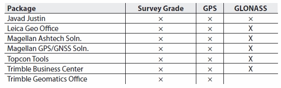
Tab. 3: Exemplary GNSS survey processing packages.
Positioning software packages can typically import two or more types of GNSS receiver data. A receiver’s native format is usually a proprietary format that a manufacturer has developed for a number of receiver models from a production line, such as those used for high-end or geodetic quality positioning. Software products developed by receiver manufacturers usually import and process data in the proprietary format. However, if GNSS data from different brands of receivers are to be processed, then for the most part, a utility program will need to convert the data to a common format before being imported.
One of the most common formats for GNSS data processing is RINEX (Gurtner and Mader, 1990) which is an acronym for Receiver Independent Exchange format (see Appendices B.13–16). GNSS survey campaigns often have many stations with numerous receiver and antenna combinations from several manufacturers. One of the easiest approaches is to work with the data in a common format. The second benefit to using RINEX data is that it is an ASCII format so a user can easily view the GNSS observations and other metadata in the RINEX file. A very good and freely available tool for converting manufacturers’ native receiver formats to RINEX is TEQC which was developed and is maintained by UNAVCO, a non-profit membership-governed consortium which facilitates geoscience research and education using geodesy. The TEQC utility, documentation and a tutorial can be downloaded from the web site listed in Appendix B.19.
There are also a limited number of high end processing packages which have been developed by government and academic institutes over that last decade. These packages offer sophisticated processing techniques and algorithms and are primarily used to process GNSS data from small and large networks collected under a variety of conditions. These programs are also used for satellite orbit determination by several IGS analysis centers on a daily basis.
Since this report primarily pertains to cost-effective GNSS, the main question that arises is how to economize ones financial and physical resources without losing quality. In general a surveyor has to work as accurately as necessary to meet the requirements given by the principal, not as accurate as possible. In other words, efficient technologies and techniques should be used to generate well-qualified products which meet the needs of the surveyors. Within this report, two possibilities to economize resources will be described in more detail.
The first possibility (see Section 4.3) is the use of Continuously Operating Reference Stations (CORS) or even CORS networks. In this case, the expenses for the master or reference station can be avoided. This implies that the costs for the hardware as well as the salaries for staff to operate the reference station may be saved. Besides, the organizational effort is reduced significantly since the surveyor may act as though he performs an absolute GNSS survey. In most countries, the surveyor usually pays for PDGNSS services provided by CORS network service provider or authority. Nevertheless the benefit provided is often enormous.
The second possibility (see Section 4.2) is to use GNSS receivers and antennas that are less expensive than “standard” geodetic equipment. The utilized receivers may be navigation or resource grade receivers or even OEM-boards or small GNSS or GPS modules. These types of receivers have low prices which start at around 150 €. Users may economize the price difference to a geodetic receiver, if he knows how to handle the respective hardware and software. These types of receivers may be used in combination with a CORS network in real time as a rover receiver to combine the two price advantages.
Normal geodetic GNSS surveys are based on high-quality GNSS receivers and antennas. Frequently, the surveying community uses dual-frequency receivers to solve the ambiguities faster and more reliably. In the last few years, single-frequency receivers have proved to work very reliably if baseline lengths are below 10 km to 15 km. This opens up the market for receivers that are used for navigation since these receivers generally have a single frequency.
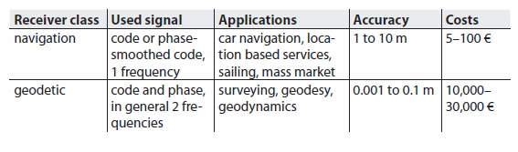
Tab. 4: Characteristics of geodetic and navigation GNSS.
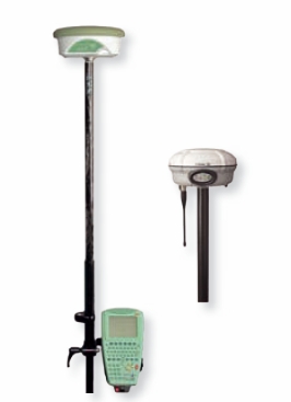
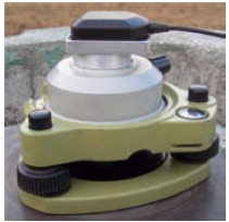
Fig. 6: Exemplary geodetic receivers.
Table 4 compares the characteristics between navigation and geodetic quality receivers. In general navigation type receivers do not use the phase data. This problem is overcome by some manufactures where they provide access to the code and phase measurements from the raw via a serial or a USB interface. Some of manufacturers (e.g. u-blox) are officially documenting their format while others (e.g. Garmin) do not provide official format information or guarantee that the format will exist in the future. Finally, some manufacturers (e.g. Sirf ) document their phase data format but do not provide access to the data for the users. With respect to geodetic quality receivers, a real time solution cannot be provided. Currently the raw carrier phase and code data are transformed into RINEX data and stored before it can be used efficiently. For the u-blox Lea-4T, the conversion from raw to usable observables may be carried out using the software teqc (see Appendix B.19).
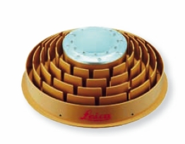
For geodetic applications, highly precise antennas such as the micro-strip and choke rings are commonly used. They are constructed to reduce multipath effects and phase centre variations as well as type specific variations regarding the antenna phase centre offset. These choke ring antennas may cost up to 10,000 €. Sometimes the GNSS receiver and antenna are integrated as one unit. In contrast, many navigation type receivers integrate low-priced, simple antennas directly into their receiver box, while some receivers simply connect to an external antenna via a cable. In the latter case, the antenna may be fixed such as on the roof of a car using a magnet on the antenna casing. Portable antennas usually range in price but start at several €s or $s. In general however, an antenna and a receiver are sold as a package.
The quality of the performance of navigation type receivers can be improved if precise geodetic antennas are used. In this example, the cost-effectiveness is clearly reduced, so in this report the combination of navigation type receiver and navigation type antenna is mainly considered. The advantage of precise geodetic antennas can be reduced or even eliminated if the navigation type antennas are calibrated. Figure 11 shows an example for the u-blox ANN-MS antenna (in combination with the u-blox LEA 4T receiver). Additionally, the navigation antennas need the capability of being leveled and centered. Figure 10 shows an adapter that combines geodetic style equipment, such as the Leica tribrack, with a u-blox ANN-MS antenna. Some experiments show that metal ground plates often reduce multipath effects, especially when metal reflectors such as a car roof are nearby.
|
|
|
|
|
|
In the following section, an overview on low-cost, receiver-antenna combinations are given. The entries in the table are given as an example, mainly because the content and number of combinations in the table will change rapidly in the future. The overview is restricted to exemplary Garmin and u-blox receivers for prices up to 150 € for a receiver-antenna combination. Garmin offers more receiver types which provide phase data in a documented or non-documented way.
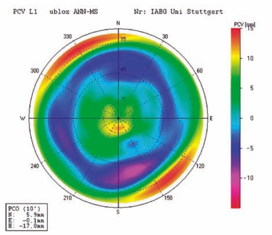
Fig. 11: Antenna pattern for u-blox ANN-MS antenna.
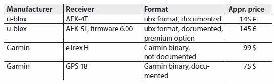
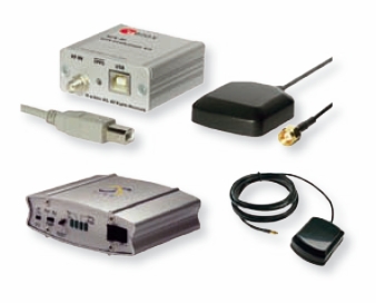
Tab. 5: Overview on low-cost GNSS receivers with available phase data.
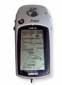
The accuracy of coordinates determined by low-cost receivers is very similar to those obtained from geodetic type receivers. Hill et al. (2001) reports standard deviations below the dm level for Garmin receivers. Schwieger documents accuracies around 2 cm for baselines up to 1.1 km using a Garmin eTrex receiver (Schwieger, 2007 and Schwieger & Wanninger, 2006) and below 2 cm for baselines up to 7 km using a u-blox AEK-4T receiver (Schwieger, 2009) with observation times between 20 and 30 minutes.
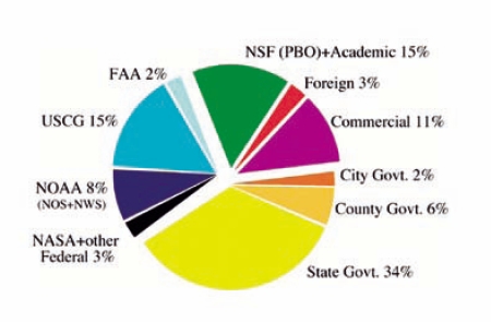
Fig 12: Federal, state, local, commercial and academic participants of
the CORS network in the United States.
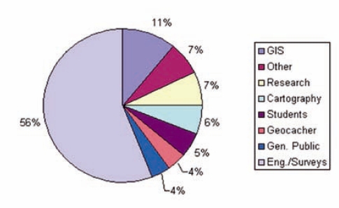
Fig 13: Sectors who use GNSS data on a routine basis.
ABIDIN & MUCHLAS (2005) obtain standard deviations below 20 cm for baselines up to 100 km in length with 20 minutes occupation time. In conclusion, the accuracy is not equivalent to single- or dual-frequency geodetic receivers but for many surveying applications the level is sufficient.
In 1994, William E. Strange, the Chief Geodesist of the National Geodetic Survey, was the first individual who defined the term Continuously Operating Reference Station (CORS) as a permanently installed geodetic quality receiver and antenna positioned over a monument or point which collected GPS data 24 hours a day, every day of the year. The initial idea was to establish a network of CORS so users could use data from any of the permanent stations with their own GPS equipment. CORS networks typically have GNSS receivers which provide carrier phase and code range measurements in support of 3-dimensional positioning activities. Today there are numerous CORS networks which have been established throughout the world (see Appendix C) to support an unlimited number of applications.
Engineers, surveyors, GIS/LIS professionals, scientists and others can apply CORS data to position points at which GNSS data have been collected as well as using the data to model a number of physical systems. A CORS system enables positioning accuracies that approach a centimeter or better relative to a worldwide network, such as the ITRF or to a local network such as the NAD83 in the United States. CORS systems benefit from a multi-purpose cooperative endeavor involving numerous governmental, academic, commercial and private organizations. As an example, the diagrams shown below illustrate the agencies and sectors that participate in the National CORS network of the United States.
The size and complexity of a CORS network varies considerably and therefore one station design cannot address all configurations. However, the following areas should be considered when planning new CORS or expanding an existing network. GNSS receivers should be able to track multiple constellations such as simultaneously collecting data from the GPS and GLONASS systems. The receiver should also use a geodetic quality antenna, preferably one that minimizes multipath and is mounted to a pillar or other stable structure. For remote installations, an enclosure to house power supplies, batteries, a computer and telecommunications equipment is strongly suggested. If the CORS station is part of a mission-critical program such as the Wide Area Augmentation System (WAAS) offered by the Federal Aviation Administration (FAA), then installing multiple receivers at a location is worth considering. The following figure below depicts a typical CORS installation from the Plate Boundary Observatory (PBO) in the Western United States.
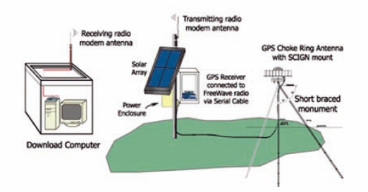
Fig 14: Typical CORS station configuration for the Plate Boundary
Observatory (PBO) network. Courtesy UNAVCO, CO.
For large CORS networks, the design may include regional data centers for quality checking, processing, distributing and archiving GNSS data. Most networks around the world collect and disseminate GNSS data 24 hours a day as well as offering other services and IGS products such as broadcast and precise ephemerides and clock information for post processing (see Appendix A).
There are also an increasing number of data centers which offer real time RTCM-104 format data streams using the Networked Transport of RTCM via Internet Protocol (Ntrip) (see Appendix B.6, B.10). Ntrip is an open protocol based on the Hypertext Transfer Protocol HTTP/1.1 and has many advantages such as having the ability to stream any kind of GNSS data, disseminating numerous streams simultaneously and can be used over mobile IP networks using TCP/IP. Data centers which offer RTCM or real time data streams usually have a server known as an NtripCaster that listens for requests from users NtripClients for one or more data streams. The data streams are then used to support stationary or mobile applications such as rapid static and kinematic surveys, hydrography, LIS/GIS development and vehicle navigation. These types of data centers will play a more significant role as the need for faster and more readily available GNSS information is desired.
A rapid and automated use of CORS networks are implemented in many post-processing services. In this case, a user does not need to worry about the processing tasks involved. A user sends their data, usually in RINEX format, to the service provider, a solution is computed and the estimated coordinates are sent to the user via email. The following sections will give an overview of four different services that are currently available for use.
The Online Positioning User Service (OPUS) from the National Geodetic Survey is a web-based service to provide GPS users with an easy method to submit and process their data in an accurate and reliable fashion. The end products are two sets of geodetic coordinates having a precision of about 1.0 cm and are consistent with the latest ITRF coordinate system and the National Spatial Reference System (NSRS) of the United States.
To use OPUS, a user needs to provide the name of the raw or RINEX data file, select an antenna type from a pull-down menu, enter the antenna height and provide an email address to which the report will be mailed. Once the data has been upload and verified, a web page reports the data has been submitted successfully and a user should expect his or her results via email a few minutes later. OPUS then uses L1 and L2 carrier phase data from the rover and the best three CORS stations in the vicinity of the rover for processing. The CORS stations are usually from the National CORS network if a rover dataset was collected in the United States or from the IGS network if the rover was collected in a foreign country or region.
OPUS relieves users of the burden of processing their own data by providing a simple interface and rapid turnaround. The service processes about 20,000 datasets a month and has over 60,000 unique users. OPUS has been used to support numerous applications with a few of the most popular being to support construction and engineering projects, surveying, mapping, mining and spaced-based imagery.
To learn more about OPUS or begin using the services offered by the National Geodetic Survey, please visit the web page listed in Appendix B.23.
The Scripps Coordinate Update Tool (SCOUT) is also a web-based geodetic tool that can be used to compute a set of coordinates for a station. SCOUT assumes the data is submitted in RINEX format which could be normal or Hatanaka-compressed observation files that may be further compressed using the traditional UNIX compress, gzip or bzip utilities.
SCOUT uses the GAMIT processing engine from the Department of Earth Atmospheric and Planetary Sciences, MIT to process the submitted dataset with CORS data from the three closest stations. A least squares network adjustment is performed with the rover and CORS and upon completion, coordinates, statistics and a regional map which shows the location of the stations are emailed to the user. The Cartesian coordinates are referenced to the ITRF05 reference frame while the geodetic coordinates are referenced onto the World Geodetic System 1984 (WGS84). For additional information on the SCOUT program offered by the Scripps Orbit and Permanent Array Center, Scripps Institute of Oceanography, please see the web link at Appendix B.24.
AUSPOS is also a web-based positioning utility which provides users the ability to submit GPS data to a processing system. This free service accepts static, dual frequency, geodetic quality data and makes use of the Geocentric Datum of Australia (GDA) and the International Terrestrial Reference Frame (ITRF). AUSPOS also uses a number of IGS products in the processing phase to produce an accurate and consistent set of coordinates for data collected anywhere on the globe.
AUSPOS has been specifically tailored to simplify several surveying and engineering tasks such as positioning DGPS and remote GPS reference stations, determining ultralong GPS baselines, establishing geodetic connections to IGS and ARGN stations and for performing GPS network quality control. To use the service, a user typically submits the antenna type and height, an email address and RINEX data, up to 24 hours in duration, to a website for processing. A set of the closest IGS reference stations are then used in a double difference approach to estimate the best set of coordinates for the remote dataset while holding the remaining IGS stations fixed. The results are provided in an email as well as through a link to the AUSPOS anonymous ftp server which stores the results. For additional information on AUSPOS, please visit the web address referenced in Appendix B.25
Natural Resources Canada (NRCan) provides a precise point positioning (PPP) service through the web which can compute highly accurate positions from raw GPS observation data in a post-processing mode. The PPP system uses precise IGS orbit and clock information and can accept static or kinematic data from either single or dual frequency receivers. The processing algorithm determines what observables are available and then proceeds with one of two scenarios. The first approach is to use L1 and L2 pseudorange and carrier phase data to obtain a solution. If the first approach fails or if the data only contains a single frequency, then an L1 pseudo-range solution will be performed.
The PPP processing system was designed to simplify GPS processing by providing a minimum number of requirements to address. A user needs to submit a RINEX file, select the type of processing desired and the reference frame the coordinates are to be reported in. Currently the PPP service will produce coordinates referenced either to the NAD83 (CSRS) or to the ITRF systems. A successful solution will produce an email sent to the user which contains a link to two forms of output. The summary reports can be short or extended and contain statistical information as well as the coordinates. A time series plot containing the estimated parameters and corresponding standard deviations is also available for review and downloading. For more information on NRCan’s PPP system, please refer to the web link in Appendix B.26.
After a description of the technical details given in the proceeding chapters, this chapter highlights the economic benefits associated with the reduction of the working costs by implementing the techniques described before. The estimation of the financial benefit cannot be 100% correct since the labor costs are quite different in most countries. For this reason, approximated values and intervals are introduced and shown in the following figures. We use an interval from 1 € (lowest level, developing countries) to 70 € (developed countries) to get a rough estimation.
As a first example, the benefit of a using a CORS reference station network is presented. For this variant, the surveyor economizes the financial resources to be spent for the receiver at the reference site and for one person to assemble and care for the reference receiver during the measurement stage of the survey. Geodetic dual-frequency receivers having a price of 20,000 € are used for the comparison. It is assumed that a receiver can be used for three years and would therefore give a 6,666 € per year operational cost. Two variants could be investigated. The first is when the service is free of charge and the second is when you have to pay for it. For the second case an interval from 500 € up to 3,000 € per year as possible flat rates may be considered. Figures 16, 18 and 19 reflect a flat rate of 1,000 € per year. Figure 15 shows the costs per year for the case where no cost-effective techniques are used. Figure 16 presents the case where the costs of integrating the receiver into a CORS network are considered. For both figures, the costs are estimated for different labor costs which range from 1 € and 70 € per hour.
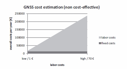
Fig 15: Costs per year for geodetic positioning using GNSS standard
configuration.
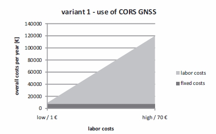
Fig 16: Costs per year for geodetic positioning applying CORS
integration.
The second benefit is achieved when low-cost receivers are used for data acquisition. In this case, the amount for the rover and the reference receiver is reduced significantly, usually between 20,000 € to approximately 100 €. The labor costs do not change, but there may be additional costs such as for two laptop computers or data loggers (overall approximately 2,000 € in 3 years) have to be considered. Software is an additional expense and is available for 1,000 €. Figure 17 presents the costs for this variant.
The third possibility is the combination of both, the use of low-cost receivers with a CORS network. For this variant shown in figure 18, the assumptions given above are still valid.
Obviously Figures 15 through 18 make it difficult to visualise what effect different labor costs have. Figure 19 therefore illustrates the benefits of the different variants (Figures 16–18) with respect to the GNSS standard configuration (Figure 15) for three labor cost levels (1 €, 10 € and 70 €). The benefits and cost savings in using a CORS station or network is important in many cases, but for developed countries it is most beneficial because labor costs are high and these are the ones to be optimized in this variant. Variant 2 is most important for very low labor costs but becomes less attractive with increasing labor costs, especially when they are given as a percentage. The benefit is further improved for the combination of both variants.
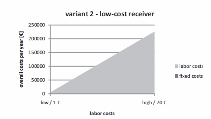
Fig 17: Costs per year for geodetic positioning using Low-Cost GNSS.
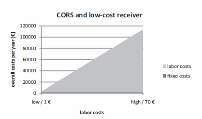
Fig 18: Costs per year for geodetic positioning using CORS and Low-Cost
GNSS.
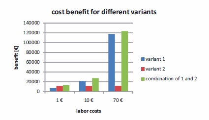
Fig. 19: Benefit of the different cost-effective techniques.
FIG Commission 5 – Positioning and Measurement would like to emphasize that there are many possibilities when performing static and kinematic surveys and are encouraged by the results delivered by current GNSS positioning technologies. The reliability, promptness and accuracy of the hardware and techniques will continue to increase in the future, especially when the number of available satellites continues to grow from year to year.
The main focus of the report was to describe the use of this emerging technology in a cost-effective way and to illustrate the cost advantages of these technologies. The advantages shown will hopefully encourage surveyors all over the world to establish cost-effective surveying practices using GNSS positioning within their profession.
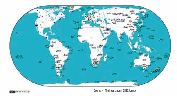
The International GNSS Service (IGS) is a voluntary scientific organization which was officially founded in January 1994. The IGS, originally known as the International GPS Service, was renamed in 2005 because other operational (GLONASS) and planned (Galileo) Global Navigation Satellite Systems (GNSS) were increasingly playing a more significant role. Today the IGS is a service of the International Association of Geodesy (IAG) and consists of more than 200 participating organizations from approximately 80 countries whose primary mission is to collect, archive and disseminate high-quality GPS and GLONASS data and associated products (Beutler et al. 1999, 2009, Dow et al. 2009).
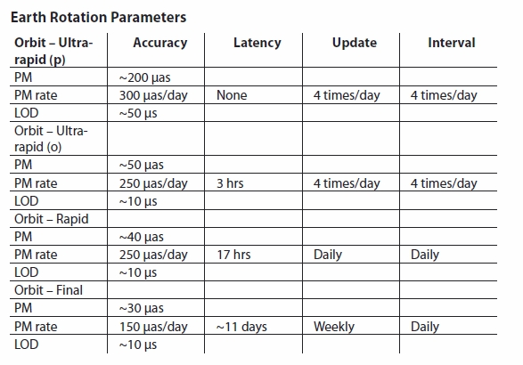
Many of the products offered through the IGS are derived from satellite observation data taken directly from the global IGS tracking network. As of May 2009, approximately 300 continuously operating reference stations (CORS) form the network, with many of the stations providing data in real-time or near real-time to a central processing center. The data are then used to compute precise and highly accurate geodetic measurements to support numerous scientific fields such as geodesy, geodynamics, engineering, oceanic and atmospheric research, navigation, and surveying and mapping. The first few products to become freely available from the IGS were the GPS satellite ephemerides, GPS clock corrections and the earth rotation parameters (ERP). GLONASS products started to show up during 1998 after a sufficient number of satellites were in orbit. Additional products such as troposphere and ionosphere data, reference station data in RINEX format (Gurtner et al. 1990, 2002), reference station coordinates and velocities were added later and are now freely available through the IGS Central Bureau (see http://www.igs.org/components/prods.html) and several global and regional analysis centers. Although the majority of the products produced are used by academic and research institutes for scientific investigations, several products such as satellite ephemerides and RINEX data are heavily used by the engineering and surveying communities. These types of data are also compatible with numerous third party GIS, engineering and surveying software products and are used in many different applications.
Today numerous users have adopted many of the IGS products for use in cm-level geodetic positioning applications as well as using the products for maintaining a highly accurate International Terrestrial Reference Frame (Altamimi et al. 2009). Users will continue to benefit from the improvements and timeliness of these products as more accurate positioning and navigation applications become part of the mainstream.
Clock Products
Currently there are seven IGS analysis centers which produce clock solutions on a daily basis. Theses clock solutions are used by the IGS Clock Product Coordinator to form two IGS timescales, the new Rapid IGS timescale (IGRT) and the new Final IGS timescale (IGST). The IGS Rapid and Final products are then aligned to these timescales. For additional information on the IGS clock products, see https://timescales.nrl.navy.mil/IGStime/index.php, (Ray et al. 2003).
Real Time Pilot Project
The concept of a real time network within the IGS infrastructure
originated at a workshop titled Towards Real-Time in Ottawa, Canada in 2002.
Since that time a prototype network referred to as the Real-time Pilot Project
was developed and became operational with over 50 active stations. As of April
2009, there are two operational systems to deliver real time data to the users.
The first system, UDPRelay, is operated by Natural Resources Canada (NRCan) and
provides data streams from 50 stations using the UDP protocol. The second system
uses the Bundesamt für Kartographie und Geodäsie (BKG) NTRIP infrastructure and
transmits data from reference stations to several broadcast servers known as
NtripCasters. Data from 150 reference stations can now be accessed via the HTTP
protocol from the IGS Caster at www.igs-ip.net.
Please refer to the following web addresses for additional information on the
two real-time networks.
http://www.rtigs.net/architecture.php
http://igs.bkg.bund.de/index_ntrip.htm
Reference Frame Working Group
The Reference Frame Working Group is primarily tasked with
generating the coordinates and velocities for the reference stations in the IGS
global network, computing daily EarthRotation Parameters (ERP) and weekly
estimates for the geocenter, as well as producing the corresponding covariance
information. The computations are usually aligned to the International
Terrestrial Reference Frame (ITRF) and performed on a regular basis. Daily
solutions are routinely „stacked“ in a cumulative fashion to obtain a more
accurate set of coordinates and velocities at a specific epoch. The Reference
Frame Working Group also strives to design efficient algorithms and accurate
models to produce the best set of products for the IGS. For additional
information on IGS station products, please visit the following web page.
http://igscb.jpl.nasa.gov/projects/reference_frame/index.html
Ionosphere Working Group
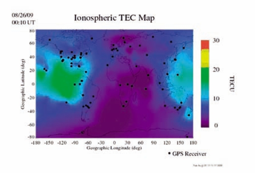
The IGS Ionosphere Associate Analysis Centers (IAAC) use varying techniques to produce independent rapid and final Vertical Total Electron Content (TEC) maps and datasets as well as producing combined versions of both products. Regional and global TEC maps are widely used by many scientific fields and commercial communications industries for monitoring the ionosphere, calibrating positioning and navigation systems and for applying corrections due to signal delays experienced from satellites above the ionosphere. The figure below was created in real time with data received from 100 global tracking sites and shows a dynamic ionosphere on August 26, 2009; Courtesy Jet Propulsion Laboratory, California Institute of Technology.
Troposphere Working Group
There are currently nine Associate Analysis Centers which are involved in producing atmospheric products related to the troposphere and the ionosphere. These two regions of the atmosphere are fairly dynamic and each can have a significant impact on GNSS signals. The main product of the Troposphere Working Group is an estimate for the total zenith path delay computed from the reference stations in the IGS global network. If additional measurements such as temperature and pressure are taken at ground level near a reference station, then it is possible to estimate the precipitable water vapor from the zenith path delays. The precipitable water vapor is of particular importance to groups working in meteorology and climatology since the quantity of water vapor in the atmosphere determines the type of weather forecast given for the next 6 to 12 hours. Longer term monitoring of water vapor from a regional point of view is also important for estimating climate change. For additional information on this topic, please visit the following web page. http://igscb.jpl.nasa.gov/projects/tropo/index.html
http://igscb.jpl.nasa.gov/network/netindex.html
The International GNSS Service (IGS).
http://www.igs.org
IGS Central Bureau (IGSCB)
http://igscb.jpl.nasa.gov/
Crustal Dynamics Data Information System (CDDIS)
http://cddis.nasa.gov/ftpgpsstruct.html
International Assocaition of Geodesy
http://www.iag-aig.org
The International Earth Rotation and Reference Systems
Service
http://www.iers.org
Networked Transport of RTCM via Internet Protocol (NTRIP)
http://igs.bkg.bund.de/index_ntrip.htm
IGS Real Time Working Group
http://www.rtigs.net/architecture.php
IGS Clock Products Working Group
https://goby.nrl.navy.mil/IGStime/
Natural Resources Canada, Earth Sciences Sector
http://ess.nrcan.gc.ca/geocan/centres_e.php
The Radio Technical Commission for Maritime Services
http://www.rtcm.org/
Earth Rotation Parameters Format
http://igscb.jpl.nasa.gov/igscb/data/format/erp.txt
IONEX: The IONosphere Map Exchange Format
http://igscb.jpl.nasa.gov/igscb/data/format/ionex1.pdf
RINEX 2: Receiver Independent Exchange Format
http://igscb.jpl.nasa.gov/igscb/data/format/rinex2.txt
RINEX 2.10
http://igscb.jpl.nasa.gov/igscb/data/format/rinex210.txt
RINEX 2.11
http://igscb.jpl.nasa.gov/igscb/data/format/rinex211.txt
RINEX 3.00
http://igscb.jpl.nasa.gov/igscb/data/format/rinex300.pdf
SINEX: Solution (Software/technique) Independent Exchange Format
http://www.iers.org/MainDisp.csl?pid=190-1100110
NAVSTAR Global Positioning System Interface Specification
IS-GPS-200D
http://www.navcen.uscg.gov/gps/geninfo/IS-GPS-200D.pdf
TEQC – The Toolkit for GPS/GLONASS/Galileo/SBAS Data
http://facility.unavco.org/software/teqc/teqc.html
UNAVCO
http://www.unavco.org/
European Space Agency – Galileo
http://www.esa.int/esaNA/galileo.html
Russian Space Agency – GLONASS
http://www.glonass-ianc.rsa.ru/pls/htmldb/f?p=202:1:9939630416051479874
Online Positioning User Service – OPUS
http://www.ngs.noaa.gov/OPUS/
Scripps Coordinate Update Tool – SCOUT
http://sopac.ucsd.edu/cgi-bin/SCOUT.cgi
Online GPS Processing Service – AUSPOS
http://www.ga.gov.au/geodesy/sgc/wwwgps/
Canadian Spatial Reference System – PPP
http://www.geod.nrcan.gc.ca/products-produits/ppp_e.php
IGS Tracking Network
http://igscb.jpl.nasa.gov/network/netindex.html
The National CORS Network – United States
www.ngs.noaa.gov/CORS/
Plate Boundary Observatory – Western United States
http://pboweb.unavco.org/
The Southern California Integrated GPS Network
http://www.scign.org/
The Western Canada Deformation Array
http://gsc.nrcan.gc.ca/geodyn/wcda/index_e.php
The Canadian Spatial Reference System
http://www.geod.nrcan.gc.ca/cacsname_e.php
Bay Area Deformation Array – USGS/UC Berkeley
http://www.ncedc.org/bard/
Eastern Basin-Range and Yellowstone Hotspot GPS Network
http://www.earth.utah.edu/people/faculty/rsmith
Pacific Northwest Geodetic Array
http://www.panga.cwu.edu/
Parkfield, California Crustal Deformation Measurements
http://earthquake.usgs.gov/research/deformation/monitoring/
Red Geodésica Nacional Activa – Mexico
http://www.inegi.org.mx/inegi/default.aspx?s=geo
Estaciones GNSS Permanentes – Argentina
http://www.copa.org.ar/Eljalon/estaciones.htm
SAPOS ® – German National Survey Satellite Service
Positioning in Berlin
www.stadtentwicklung.berlin.de/geoinformation/sapos/
SWEPOS – Swedish Network of Permanent Reference Stations for GNSS
http://swepos.lmv.lm.se/
EUREF Permanent Network – Europe
http://www.epncb.oma.be/_trackingnetwork/
Geodetic Data Archiving Facility – Italy
http://geodaf.mt.asi.it/html_old/index.html
Réseau GPS Permanent – France
http://rgp.ign.fr/
Automated GNSS Network for Switzerland
http://www.swisstopo.admin.ch/internet/swisstopo/en/home/topics/survey/permnet/
agnes.html
CZEPOS – Czech Republic
http://czepos.cuzk.cz/
ESTPOS – Estonia
http://www.maaamet.ee
GPSNET.HU – Hungary
http://www.gpsnet.hu
LATPOS – Latvia
http://www.latpos.lgia.gov.lv
LITPOS – Lithuania
http://eupos.vgtu.lt/
ASG-EUPOS – Poland
http://www.asg-eupos.gov.pl
ROMPOS – Romania
http://www.rompos.ro
AGROS – Serbia
http://www.agros.rgz.gov.rs
SKPOS – Slovak Republic
http://www.skpos.gku.sk
SIGNAL – Slovenia
http://www.gu-signal.si
Geographical Survey Institute – Japan
http://www.gsi.go.jp/ENGLISH/page_e30030.html
Australian Regional GPS Network
http://www.ga.gov.au/geodesy/argn/
GeoNet – New Zealand
http://www.geonet.org.nz/index.html
PositioNZ – New Zealand
http://www.linz.govt.nz/geodetic/positionz/index.aspx
Published in English
Copenhagen, Denmark
ISBN 978-87-90907-79-2
Published by
The International Federation of Surveyors (FIG)
Kalvebod Brygge 31–33, DK-1780 Copenhagen V
DENMARK
Tel. +45 38 86 10 81
Fax +45 38 86 02 52
E-mail: FIG@FIG.net
www.fig.net
January 2010
ACKNOWLEDGEMENTS
Editors: Dr. Neil D. Weston, United States and Dr. Volker Schwieger, Germany
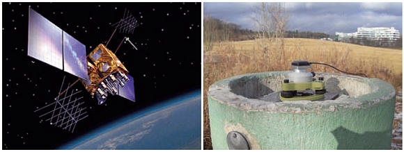
Cover photos, front: GPS IIR satellite, u-blox antenna on pillar (©IAGB)
Design and layout: International Federation of Surveyors, FIG
Printer: Oriveden Kirjapaino, Finland
Cost Effective GNSS Positioning Techniques
FIG Commission 5 Publication
Published in English
Published by The International Federation of Surveyors (FIG), February 2010
Copenhagen, Denmark
ISBN: 978-87-90907-79-2
Printed copies can be ordered from:
FIG Office, Kalvebod Brygge 31-33, DK-1780 Copenhagen V, DENMARK,
Tel: + 45 38 86 10 81, E-mail:
FIG@fig.net